
*이 글을 읽기전에 작성자 개인의견이 있으니, 다른 블로그와 교차로 읽는것을 권장합니다.*
1. ROI
관심 영역(ROI, Region of Interest)
- 영상 내에서 관심이 있는 영역
cv2.selectROI()
import cv2

img = cv2.imread('./sun.jpg')

# x, y, w, h
x=182
y=21
w=122
h=110

# 태양을 복사
roi = img[y:y+h, x:x+w]
roi_copy = roi.copy()

# 오른쪽에 붙이기
img[y: y+h, x+w: x+w+w] = roi
# 두 태양을 박스로 감싸기
cv2.rectangle(img, (x, y), (x+w+w, y+h), (0, 255, 0), 3)

cv2.imshow('img', img)
cv2.imshow('roi_copy', roi_copy)
cv2.waitKey()

import cv2

oldx = oldy = w = h = 0
color = (255, 0, 0)
img_copy = None
isDrag = False

def on_mouse(event, x, y, flags, param):
    global oldx, oldy, w, h, isDrag, img_copy
    if event == cv2.EVENT_LBUTTONDOWN:
        isDrag = True
        oldx = x
        oldy = y
    elif event == cv2.EVENT_MOUSEMOVE:
        if isDrag:
            img_copy = img.copy()
            cv2.rectangle(img_copy, (oldx, oldy), (x, y), color, 3)
            cv2.imshow('img', img_copy)
    elif event == cv2.EVENT_LBUTTONUP:
        if isDrag:
            isDrag = False
            if x > oldx and y > oldy:
                w = x - oldx
                h = y - oldy
                if w > 0 and h > 0:
                    cv2.rectangle(img_copy, (oldx, oldy), (x, y), color, 3)
                    cv2.imshow('img', img_copy)
                    roi = img[oldy: oldy+h, oldx: oldx+w]
                    cv2.imshow('roi', roi)
        else:
            cv2.imshow('img', img)
            print('영역이 잘 못 되었음')

img = cv2.imread('./sun.jpg')
cv2.namedWindow('img')
cv2.setMouseCallback('img', on_mouse)
cv2.imshow('img', img)
cv2.waitKey()
import cv2

img = cv2.imread('./sun.jpg')

x, y, w, h = cv2.selectROI('img', img, False)

if w and h:
    roi = img[y: y+h, x:x+w]
    cv2.imshow('roi', roi)

cv2.waitKey()
2. Binarization
영상의 이진화(Binarization)
- 픽셀의 검은색 또는 흰색과 같이 두 분류의 값으루 나누는 작업
- 영상에서 의미있는 관심 영역(ROI)과 비관심 영역으로 구분할 때 사용
- 예) 배경과 객체를 둘로 나눌 때
- 영상의 이진화 연산을 할 때, 나누는 특정값을 임계값이라고 함
cv2.threshold()
cv2.THRESH_BINARY : 픽셀값이 임계값을 넘으면 최대값으로 지정하고 넘지 못하면 0으로 지정
cv2.THRESH_BINARY_INV : THRESH_BINARY의 반대
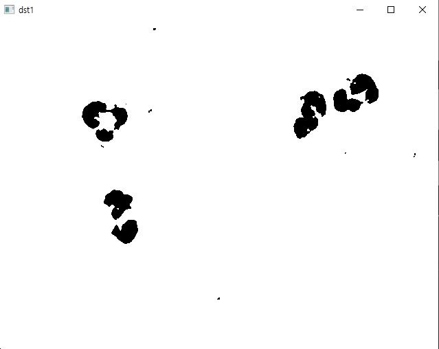
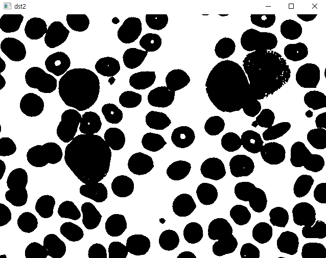
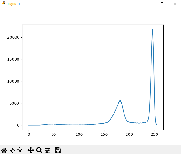
import cv2
import matplotlib.pyplot as plt

img = cv2.imread('./cells.png', cv2.IMREAD_GRAYSCALE)
hist = cv2.calcHist([img], [0], None, [256], [0,255])

# cv2.THRESH_BINARY : 픽셀값이 임계값을 넘으면 최대값으로 지정하고 넘지 못하면 0으로 지정
a, dst1 = cv2.threshold(img, 100, 255, cv2.THRESH_BINARY)
a, dst2 = cv2.threshold(img, 210, 255, cv2.THRESH_BINARY)
print('a:',a)

cv2.imshow('img', img)
cv2.imshow('dst1', dst1)
cv2.imshow('dst2', dst2)

plt.plot(hist)
plt.show()
cv2.waitKey()
3. Otsu
오츠의 이진화 알고리즘
- 자동 이진화 알고리즘
- 자동으로 임계값을 구해줌, 임계값을 구분하는 가장 좋은 방법으로 사용
cv2.threshold(영상, 임계값, 최대값, 플래드 | cv2.THRESH_OTSH)
- 임계값을 임의로 정해 픽셀을 두 부류로 나누고 두 부류의 명암 분포를 구하는 작업을 반복하여 모든 경우의 수 중에서 두 부류의 명암 분류가 가장 균일할 때의 임계값을 선택
import cv2
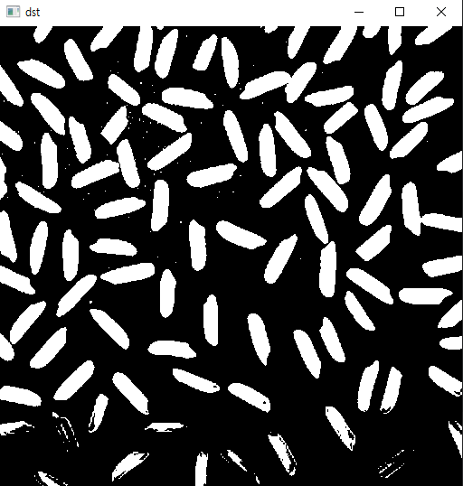
img = cv2.imread('./rice.png', cv2.IMREAD_GRAYSCALE)
th, dst = cv2.threshold(img, 0, 255, cv2.THRESH_BINARY | cv2.THRESH_OTSU)
print('otsh:', th)
cv2.imshow('img', img)
cv2.imshow('dst', dst)
cv2.waitKey()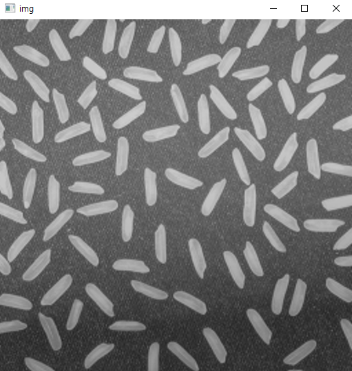
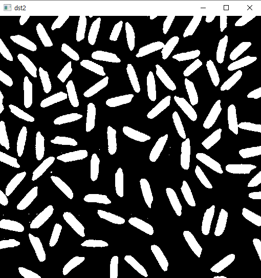
지역 이진화
- 균일하지 않은 조명 환경에서 사용하는 이진화 방법
- 전체 구역을 N등분하고 각각의 구역에 이진화를 한 뒤에 이어 붙이는 방법
- 여러개의 임계값을 이용할 수 있음
# rice.png 영상을 이용하여 가로 4등분, 세로 4등분하고 자동 이진화를 적용해보자
# 전역(자동) 이진화와 비교
import cv2
import numpy as np

img = cv2.imread('./rice.png', cv2.IMREAD_GRAYSCALE)

# 전역 자동 이진화
_, dst1 = cv2.threshold(img, 0, 255, cv2.THRESH_BINARY | cv2.THRESH_OTSU)

# 지역 이진화
dst2 = np.zeros(img.shape, np.uint8)
bw = img.shape[1] // 4
bh = img.shape[0] // 4

for y in range(4):
    for x in range(4):
        img_ = img[y*bh: (y+1)*bh, x*bw: (x+1)*bw]
        dst_ = dst2[y*bh: (y+1)*bh, x*bw: (x+1)*bw]
        cv2.threshold(img_, 0, 255, cv2.THRESH_BINARY | cv2.THRESH_OTSU, dst_)

cv2.imshow('img', img)
cv2.imshow('dst1', dst1)
cv2.imshow('dst2', dst2)
cv2.waitKey()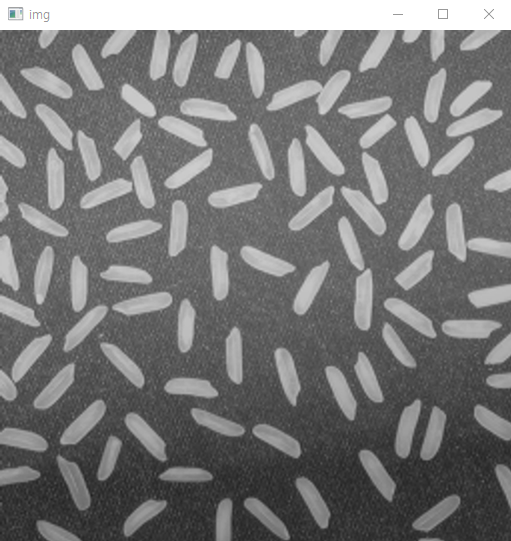

적응형 이진화
- 영상을 여러 영역으로 나눈 뒤, 그 주변 픽셀값만 활용하여 임계값을 구함
- 노이즈를 제거한 뒤에 Otsu 이진화를 적용
cv2.adaptiveThreshold()
cv2.ADAPTIVE_THRESH_MEAN_C : 이웃 픽셀의 평균으로 결정, 선명하지만 잡티가 많아질 수 있음
cv2.ADAPTIVE_THRESH_GAUSSIAN_C : 가우시안 분포에 따른 가중치의 합으로 결정, 선명도는 조금 떨어지지만 잡티가 적음
blocksize : 3이상의 값. 정방행렬. 블록 사이즈가 클수록 연산시간이 오래 걸림
import cv2
import matplotlib.pyplot as plt

img = cv2.imread('./sudoku.jpg', cv2.IMREAD_GRAYSCALE)

th, dst1 = cv2.threshold(img, 0, 255, cv2.THRESH_BINARY | cv2.THRESH_OTSU)

dst2 = cv2.adaptiveThreshold(img, 255, cv2.ADAPTIVE_THRESH_MEAN_C, cv2.THRESH_BINARY, 9, 5)
dst3 = cv2.adaptiveThreshold(img, 255, cv2.ADAPTIVE_THRESH_GAUSSIAN_C, cv2.THRESH_BINARY, 9, 5)

dic = {'img':img, 'dst1': dst1, 'dst2': dst2, 'dst3': dst3}

for i, (k, v) in enumerate(dic.items()):
    plt.subplot(2, 2, i+1)
    plt.title(k)
    plt.imshow(v, 'gray')

plt.show()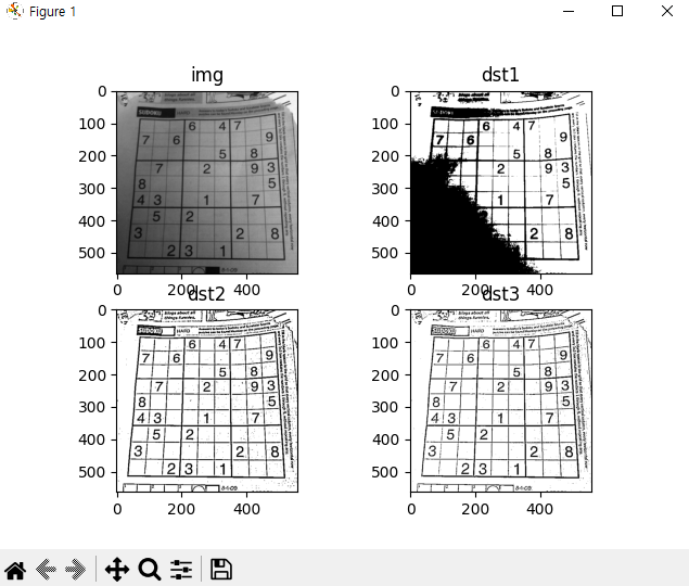
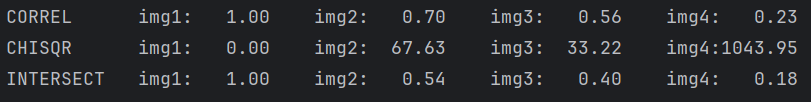
이미지 유사도
- 픽셀값의 분포가 서로 비슷하다면 유사한 이미지일 확률이 높음
cv2.compareHist()
cv2.HISTCMP_CORREL : 상관관계(1 : 완전 일치, -1 : 완전 불일치, 0 : 무관계)
cv2.HISTCMP_CHISQR : 카이제곱(0 : 완전 일치, 무한대 : 완전 불일치)
cv2.HISTCMP_INTERSECT : 교차(1 : 완전 일치, 0 : 완전 불일치)
import cv2
import matplotlib.pyplot as plt
import numpy as np

img1 = cv2.imread('./taekwonv1.jpg')
img2 = cv2.imread('./taekwonv2.jpg')
img3 = cv2.imread('./taekwonv3.jpg')
img4 = cv2.imread('./dr_ochanomizu.jpg')

imgs = [img1, img2, img3, img4]
hists = []

for i, img in enumerate(imgs):
    plt.subplot(1, len(imgs), i+1)
    plt.title('img%d' % (i+1))
    plt.axis('off')
    plt.imshow(img[:, :, ::-1])
    hsv = cv2.cvtColor(img, cv2.COLOR_BGR2HSV)
    hist = cv2.calcHist([hsv], [0, 1], None, [180, 256], [0, 180, 0, 256])
    cv2.normalize(hist, hist, 0, 1, cv2.NORM_MINMAX)
    hists.append(hist)

query = hists[0]
methods = {'CORREL': cv2.HISTCMP_CORREL, 'CHISQR': cv2.HISTCMP_CHISQR, 'INTERSECT': cv2.HISTCMP_INTERSECT}

for j, (name, flag) in enumerate(methods.items()):
    print('%-10s' % name, end='\t')
    for i, (hist, img) in enumerate(zip(hists, imgs)):
        ret = cv2.compareHist(query, hist, flag)
        if flag == cv2.HISTCMP_INTERSECT:
            ret = ret/np.sum(query)
        print('img%d:%7.2f' % (i+1, ret), end='\t')
    print()
plt.show()
'Python > 컴퓨터 비전' 카테고리의 다른 글
| Python(54)- 모폴로지 처리, 레이블링, 테서렉트 (0) | 2024.07.23 |
|---|---|
| Python(53)- 엣지 검출, 투시 변환 (0) | 2024.07.23 |
| Python(51)- CLAHE(평탄화), 색상추출, hist (0) | 2024.07.23 |
| Python(50)- OpenCV (0) | 2024.07.16 |
| Python(49)- 컴퓨터 비전 (0) | 2024.07.16 |


